Bermudan (Equity) Option (under lognormal model)

Java Applet

Alternatively you may launch this applet using Java WebStart. Minimum requirements: Java 1.6. Tested with Firefox and Safari. Source code for the underlying library is available at finmath.net.

IMPORTANT: The applet is currently self-signed. Hence it will no longer run under the Java security level "high", which has become default. In order to run the applet, you need to add the domain http://christian-fries.de to the Exception Site List. To edit the Exception Site List open the Java control panel, select the Security tab, then press Edit Site List.

Description

This tools illustrated Bermudan option pricing using Monte Carlo simulation.

It serves as a companion to Chapter 15 of Mathematical Finance.

Upon each exercise date T₁, T₂,...,T_n the holder of the Bermudan has the right to either exercise and receive N_i * (S(T_i) - K_i) or receive a shorter Bermudan option on the remaining exercises T_j> T_i. The last option pays either N_n * (S(T_n) - K_n) or nothing. Setting notional negative will give you a put instead of a call.

Evaluation Methods

Various methods to estimate the exercise boundary are implemented:

Regression: The method also known as Longstaff-Schwartz where the exercise boundary is estimated by a linear regression on some basis functions.
Binning: The definition space of the predictor variable (here the exercise value) is split into intervals (bins) on which a conditional expectation is calculated.
Threshold optimization: A root finder optimizes a scalar threshold used in a specific exercise criteria (e.g. a linear function of the intrinsic value).
Perfect foresight: The single value given by the future evolution of the path is used as "estimate" for the expectation. This gives a foresight bias an thus a wrong price (the strategy is super optimal).
Analytic: For an Bermudan with only two exercise date and a simple Black-Scholes type model the optimal exercise can be calculated analytically (using Black-Scholes Formula upon exercise).

Exercise Boundary

Figure 1: Example of the estimation of the exercise boundary.

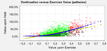
The exercise boundary is visualized in a scatter plot, see Figure 1. The picture shows the situation at a specific exercise date. Each dot represents the value upon hold depending on the value upon exercise for a specific simulation path. The conditional expectation is shown as a function of the value upon exercise (blue line). The exercise region (green) is defined as the paths having exercise values (yellow line) above the expected value upon hold (blue line).